Forecasting 2020 BIXI Rides
A little about BIXI
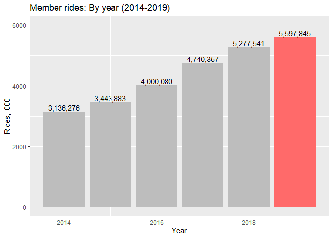
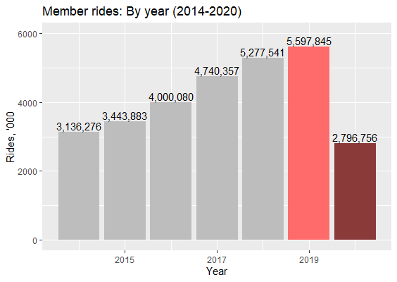
BIXI, a bike sharing service, is an organic part of the urban transit landscape in Montreal. I do think it was really smart of the city authorities to integrate bikes into the public transport network, and a proof of it is in a constantly growing number of rides taken by either BIXI members or occasional riders. The year of 2019 was a banner year for the company!
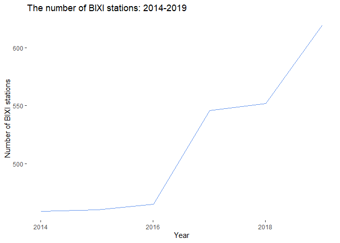
As a result of growing demand, the number of available BIXI stations is also growing, making both more bikes available for rent and opening up new routes to BIXI users.
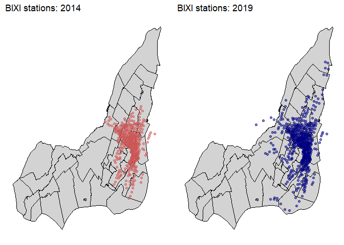
Mapping of 2014 and 2019 BIXI stations shows how BIXI expanded into the Greater Montreal area.
Task
The purpose of this analysis is to forecast a number of BIXI rides in 2020 adjusted for the COVID-19 situation.
Questions Asked
-
What are the patterns in the BIXI data?
-
Which model out of the list presented below should be used to produce the most reliable BIXI forecasts?
- Naive models (simple, seasonal and mean)
- Smoothing models (exponential smoothing, Holt’s and Winter’s)
- ARIMA
-
What would the forecasted rides be ignoring the COVID-19 situation?
-
How could the COVID-19 factors be added into the forecast?
Data and initial variables used for analysis
All 47 tables of Bixi open data (2014-2019) were used for this analysis, but only two variables were needed:
-
Date (start_date)
-
Membership (is_member)
Data transformation
1. Date transformation
Since I wanted to do a monthly forecast of BIXI rides in 2020. Using the month() function available in the libridate library, would not be enough because all rides would only be summed by months, ignoring the years. So, I would end up having only 8 rows in the output set with all April rides from 2014-2019 summed up in one cell and so on. To overcome that inconvenience, I created a synthetic date that would only be represented by the first day of each month from a given year. For example, April 2014 would be 2014-04-01 and May 2014 would be 2014-05-01.
2. Data aggregation
Both member and non-member rides were aggregated on a monthly basis per year. Since one row of the set represents a ride, the number of rows per month was calculated to get the number of trips per month per year. In addition, rides per member on a monthly basis per year were aggregated.
Challenges
- Challenge: November 2019 data missing
- Solution
On the BIXI’s site, the November 2019 table was missing. As a result, it was important to find the missing value somehow. Since the number of rides from April to October 2019 was already available on their site, all that was needed was to find a total number of rides in 2019. In their 2019 financial report, BIXI stated that the total number of rides in 2019 was 5,800,000. I used that number (which is definitely rounded, but it is better than nothing) and subtracted the number of April-October 2019 rides from it to impute the missing value.
- Challenge: BIXI data is irregular time series
- Solution
BIXI’s year only lasts for 8 months from April to November while other months’ rides equal zero. It makes it an interesting case as we do need to forecast rides within these 8 months, but we don’t need to forecast the rest of the year as we know that the number of the rides equals zero. In order not to feed those “zero-rides” months into the model, I created a “year” whose length was equal to 8 months only.
- Challenge: An increased uncertainty of 2020 forecasts due to COVID-19
- Solution
It is evident that 2020 is different from any other year in BIXI’s (and the world’s) history. A few things happened in Montreal (and in Canada and around the world) - some people lost jobs, started working or studying remotely. It could result in a decline of members’ rides. Closed borders and travel restrictions resulted in a plunge of tourism. This will definetely affect the number of occasional rides in 2020. Thus, the forecasts would need to be adjusted for that decrease.
The analysis
BIXI data was available in tables for each month for 2014 through 2019 with records collected at a time when a bike was borrowed and then returned to the station. I only had to append the tables and to extract just the start_date and the is_member variables from the master set. I spent more time, however, on creating new variables. For example, I created a variable called Rides, which represents an aggregated number of rides per date (not per datetime as was provided in the original set). All the sets used to create this post as well as the R code of the project are available on my GitHub. Feel free to go there and replicate the project!
Loading the libraries
The libraries needed for the analysis are as follows:
-
lubridate works with dates
-
forecast, smooth and zoo work with time series
-
ggplot is used to create great graphs
#Loading libraries
library(lubridate)
library(forecast)
library(smooth)
library(zoo)
library(ggplot2)
What are the patterns in the BIXI data?
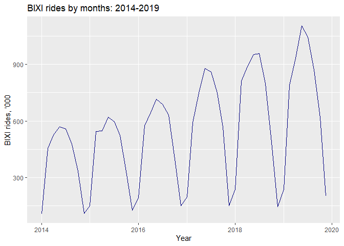
When analysing a time series data, we need to visualise it first.
As we can observe from the graph below, the data is not stationary as there is an upward trend present. In addition, the trend’s variance is increasing throughout the time. Perhaps, a Box-Cox transformation could be needed. There is also dictinct seasonality present in the data, which is expressed by the rises and falls in the graph at regular intervals year on year.
#Plotting the time series
autoplot(bixi.ts/1000, main="BIXI rides by months: 2014-2019", xlab="Year", ylab="BIXI rides, '000", color="navy")
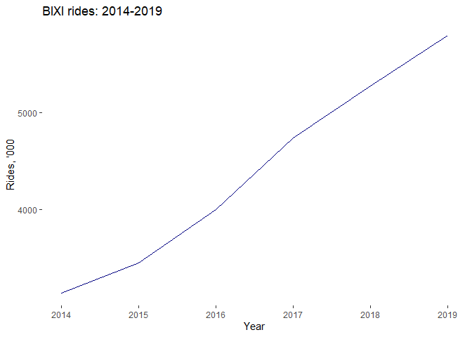
Further aggregation of the data (per year) and plotting it, made the trend more distinctive. We observe almost a straight upward line.
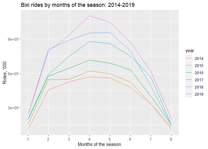
To dive further into the seasonality of the time series at hand, I created a seasonal plot. The BIXI’s year begins in April, which is represented by month=1 in the plot. We can obviously see that July has the greatest number of trips. In 2017 and 2019 July’s (month=4) rides were unusually high. It may have been caused by an increase in tourism. In 2017 both Montreal and Canada had special anniversaries to celebrate - 375 and 150 years respectively. In July 2019 soccer fans were overwhelmed with the arrival of Real Madrid to Montreal, which could have resulted in large numbers of fans coming to Montreal.
#Creating a seasonal plot of Bixi rides
ggseasonplot(bixi.ts)+ggtitle("Bixi rides by months of the season: 2014-2019")+
  xlab("Months of the season")+ylab("Rides, '000")
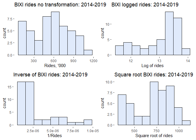
Finally, knowing more about the data, I turned to the distribution analsis of BIXI rides. Apart from checking for the distribution of the original/ regular rides, I also tried various Box-Cox transformations: logging the data, finding the inverse (1/Rides) and the square root of the rides. These resulted in highly skewed distributions either to the right (log(Rides)) or to the left (1/Rides) or in a distribution similar to the orginial rides (sqrt(Rides)). As a result, I decided to proceed with the regular non-transformed rides.
Partitioning the data
Following a conventional practice, I partitioned the data into two sets: train (4 years of data) and validation (2 years).
#Partitioning the data
nvalid <- 16 #recording a number into a vector
ntrain <- length(bixi.ts) - nvalid #the rest for 2014-2016 years - 32 observations

train.ts <- window(bixi.ts, start=c(2014,1), end=c(2014,ntrain), freq=8)
valid.ts <- window(bixi.ts, start=c(2014, ntrain+1), freq=8)
Selecting the best model
Finally, when everything was ready for analysis, I only had to set the procedure for my search for the best model to forecast 2020 BIXI rides:
1) Train the model on the train set and then forecast the validation set.
2) Compare the training and validation sets’ errors - MAPE, MPE, MSE - to check for the model’s performance and overfitting.
3) Check the residuals in both sets to see if they are random/ independent, normally distributed, have constant variance.
4) Compare models’ validation errors to each other to select the model with the best predictive power. Note: only robust models should be used for comparison.
5) Use the best naive model - simple naive, seasonal naive, simple mean - as a benchmark to evaluate other models against it. Following the parsimony principle, that states that the simpler the model is, the better; I would prefer a slightly less accurate, but less complicated model to a more accurate one that needs many more parameters. Any more complex model would need to outperform the best naive model.
Naive models
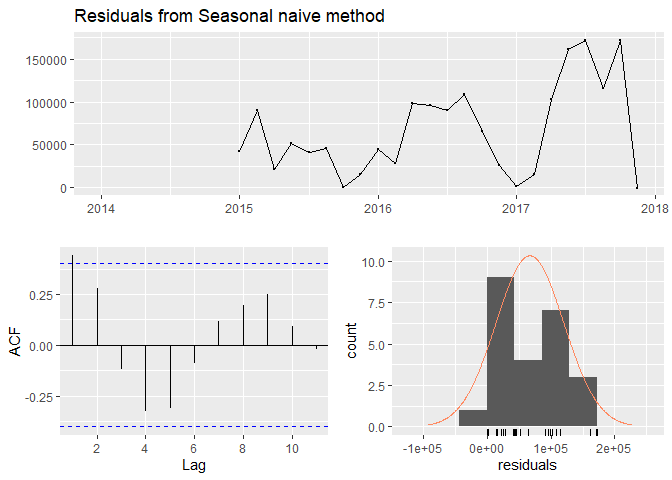
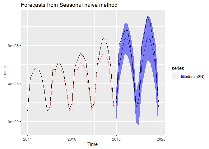
After having run three naive models - simple naive, seasonal naive and simple mean - the seasonal naive model appeared to be the best one. It seemed pretty good because of a quite small difference in error terms of the training and validation sets. In addition, its error terms were the lowest out of the three models. The residuals were correlated just at lag=1. However, the residuals were not independent. So, the model was by no means perfect, but it was used as a benchmark model. Other more complex models were later compared against it. Below I am presenting the results of fitting the seasonal naive model.
Seasonal naive
trainSN <- snaive(train.ts, h=nvalid, level=c(95))
#Checking accuracy
accuracy(trainSN, valid.ts) #checking accuracy
##                    ME      RMSE       MAE      MPE     MAPE     MASE
## Training set 66836.71  84790.82  66854.79 12.72203 12.73395 1.000000
## Test set     99801.69 131519.59 110904.19 13.15451 15.87756 1.658882
##                   ACF1 Theil's U
## Training set 0.4395506        NA
## Test set     0.5059128 0.3815288
#Checking residuals
checkresiduals(trainSN) #checking residuals, pretty good!
##
## 	Ljung-Box test
##
## data:  Residuals from Seasonal naive method
## Q* = 14.492, df = 6, p-value = 0.0246
##
## Model df: 0.   Total lags used: 6
#Plotting the values
autoplot(trainSN) + autolayer(fitted(trainSN)) +
  autolayer(valid.ts, color="black")
Smoothing models
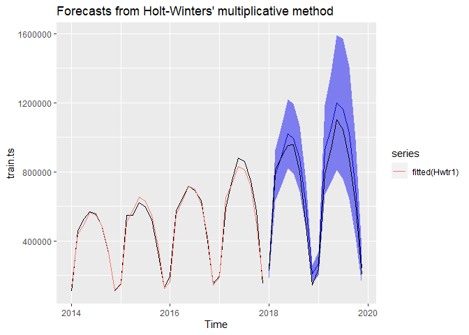
After having selected the benchmark model, I ran exponential smoothing, Holt’s, and Winter’s with additive or multiplicative seasonality. Only the best model - Winter’s Multiplicative - is presented here. The full code used to train all models and generate forecasts is available in my repository on GitHub.
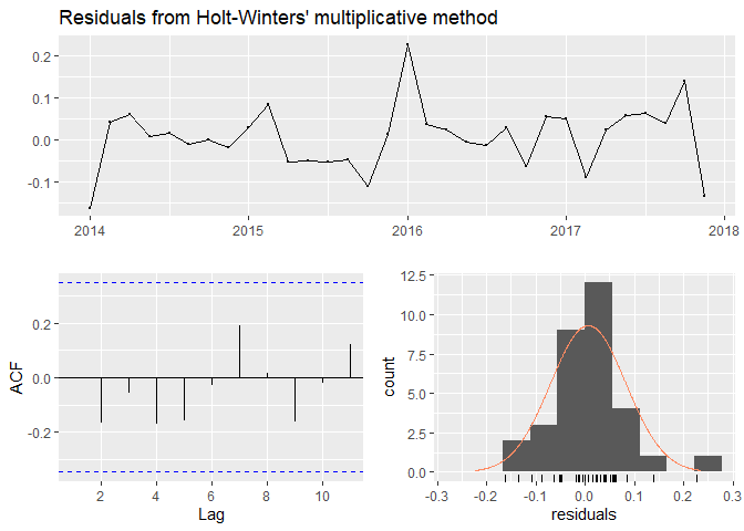
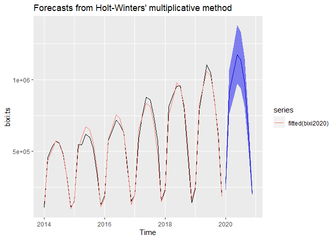
The Winter’s model with multiplicative seasonality was the best model out of all smoothing models. The code used to run the model as well as its output can be seen below. R estimated the following coefficients for the model: alpha = 0.0657, beta = 0.0657, gamma = 1e-04. This model has the lowest error terms, whose training and validation values are very close. The residuals show randomness of their distribution, they have no serial autocorrelation and are more or less normally distributed. The confidence interval boundaries include the data original values. Residuals are also very small! In addition, the model manages to forecast the training data really close to the original values. The Winter’s multiplicative is also much better than the seasonal naive model, which has much higher residuals and higher error terms.
Winter’s: Multiplicative
Hwtr1 <- hw(train.ts, seasonal="multiplicative",
           h=nvalid, level=95)
#Checking accuracy
accuracy(Hwtr1, valid.ts) #checking accuracy
##                      ME     RMSE      MAE          MPE      MAPE      MASE
## Training set   3853.463 29047.06 23250.72   0.07634078  5.659556 0.3477794
## Test set     -69029.753 86778.13 74287.00 -12.14677773 13.217462 1.1111695
##                   ACF1 Theil's U
## Training set 0.2333577        NA
## Test set     0.5356053 0.1998455
#Checking residuals
checkresiduals(Hwtr1) #checking residuals, not bad :)

##
## 	Ljung-Box test
##
## data:  Residuals from Holt-Winters' multiplicative method
## Q* = 13.657, df = 3, p-value = 0.003411
##
## Model df: 12.   Total lags used: 15
#Plotting the values
autoplot(Hwtr1) + autolayer(fitted(Hwtr1)) +
  autolayer(valid.ts, color="black")
ARIMA
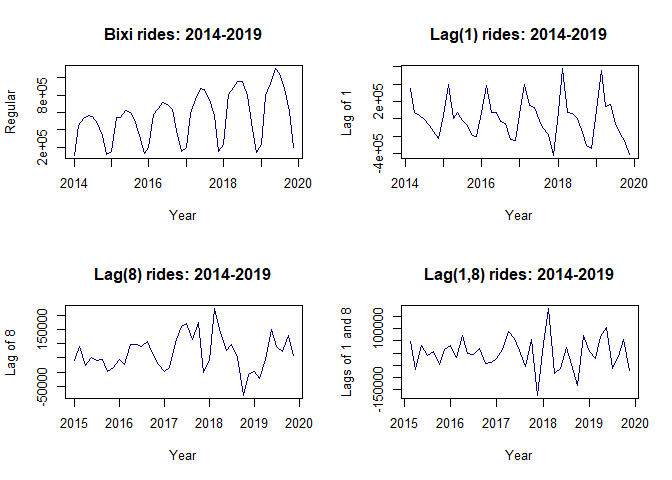
For ARIMA models it is crucial to use stationary data, especially for the moving average processes. That is a problem because our data has a distinct seasonality and a trend which also shows an increasing variance with time. That can be easily solved by differencing, though.
#differencing the data
#differencing at lag 1
lag1 <- diff(bixi.ts, lag=1)
#differencing at lag 8 (seasonal)
lag8 <- diff(bixi.ts, lag=8)
#double differencing at lag 1 and lag 8
lag1_8 <- diff(diff(bixi.ts,8),1)
We may observe that differencing the data at a lag=1 makes it more or less stationary. However, the best result can be observed when double differencing is used - at lag=1 and lag=8.
Continuing the exploration of the data before fitting ARIMA, I checked for autocorrelation of the original rides by running the Ljung-Box test. The result with its p-value being close to zero indicated that there was a serial autocorrelation present at least at up to 8 lags.
#checking for serial autocorrelations
Box.test(bixi.ts, lag=8, type="Ljung-Box")
##
## 	Box-Ljung test
##
## data:  bixi.ts
## X-squared = 95.374, df = 8, p-value < 2.2e-16
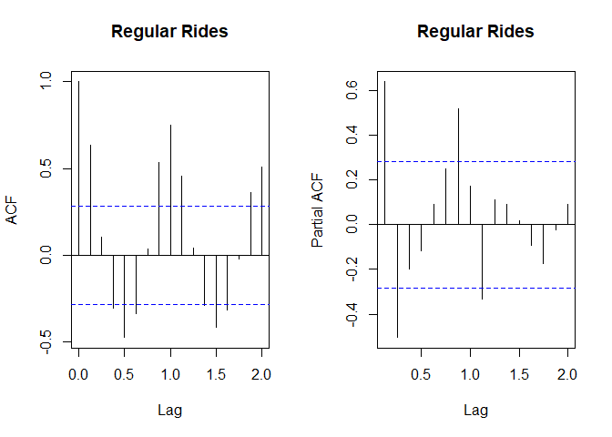
The explorations of the data were not finished yet, because it was important to investigate ACF (autocorrelations plot) and PACF (partial autocorrelations plot) to understand what ARIMA processes would need to be used. These plots were indicative of the AR underlying process. In that case, we typically observe multiple gradually subsiding autocorrelations present in the ACF plot and a few quickly subsiding partial autocorrelations (PACF plot). In addition, differencing might need to be considered, at least at lag=1.
#plotting autocorrelation plots
par(mfrow=c(1,2)) #placing 4 plots in one window
acf(bixi.ts, main="Regular Rides") #autocorrelation plot
pacf(bixi.ts, main="Regular Rides") #partial autocorrelation plot
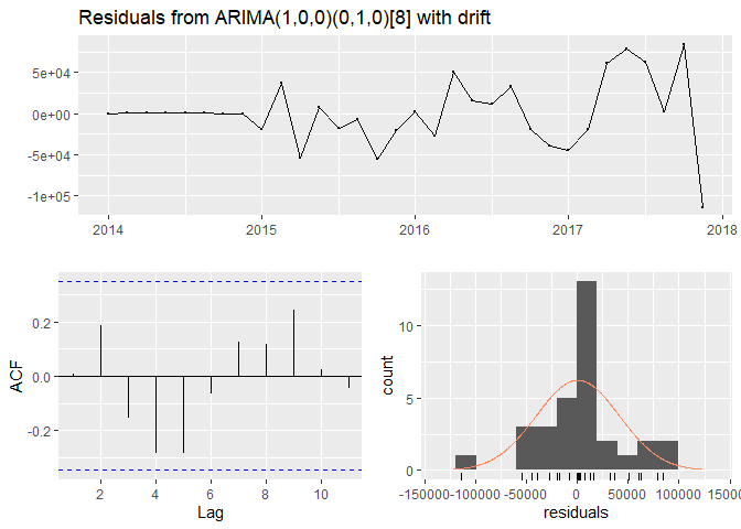
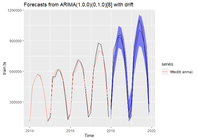
I tried multiple models: ARIMA(1,0,0), ARIMA(1,1,0), and seasonal and non-seasonal Auto-ARIMA. The best model was the one automatically selected by R - ARIMA(1,0,0)(0,1,0)[8] with a drift. It did have the lowest error terms out of all fitted ARIMA models. In addition, the distance between the errors for the training and validation data was not large, which was indicative of no data overfitting and the model’s consistent performance for both training and validation data. The residuals did not seem to show any particular patterns, but they were very high and their variance was not constant. On the other hand, the forecasts followed the data closely and the confidence interval included the actual data, which could result in a more or less accurate forecast for 2020. The model’s output is presented below.
Auto ARIMA: Seasonal
tr.arima <- forecast(auto.arima(train.ts), h=nvalid, level=c(95))
##                      ME     RMSE      MAE       MPE      MAPE      MASE
## Training set   477.2609 40153.50 27729.11 -4.021464  8.191555 0.4147663
## Test set     10858.2300 80976.83 66759.55 -5.325653 14.186127 0.9985755
##                     ACF1 Theil's U
## Training set 0.005979721        NA
## Test set     0.479017515 0.2662769
##
## 	Ljung-Box test
##
## data:  Residuals from ARIMA(1,0,0)(0,1,0)[8] with drift
## Q* = 8.6828, df = 4, p-value = 0.06954
##
## Model df: 2.   Total lags used: 6
The best model
The search for the best model was almost over. But which model was the winner? The seasonal naive? The Winter’s or the Auto-ARIMA? To answer those questions, I compared all error terms. The two best models were Holt-Winter’s multiplicative and the Auto-ARIMA. They both had much lower error terms than the seasonal naive. I considered them for the next round of comparison.
#Checking accuracy
#Seasonal Naive
accuracy(trainSN, valid.ts)
##                    ME      RMSE       MAE      MPE     MAPE     MASE
## Training set 66836.71  84790.82  66854.79 12.72203 12.73395 1.000000
## Test set     99801.69 131519.59 110904.19 13.15451 15.87756 1.658882
##                   ACF1 Theil's U
## Training set 0.4395506        NA
## Test set     0.5059128 0.3815288
#Holt-Winter's multiplicative
accuracy(Hwtr1, valid.ts) #checking accuracy THE BEST
##                      ME     RMSE      MAE          MPE      MAPE      MASE
## Training set   3853.463 29047.06 23250.72   0.07634078  5.659556 0.3477794
## Test set     -69029.753 86778.13 74287.00 -12.14677773 13.217462 1.1111695
##                   ACF1 Theil's U
## Training set 0.2333577        NA
## Test set     0.5356053 0.1998455
#AutoARIMA
accuracy(tr.arima, valid.ts) #checking accuracy
##                      ME     RMSE      MAE       MPE      MAPE      MASE
## Training set   477.2609 40153.50 27729.11 -4.021464  8.191555 0.4147663
## Test set     10858.2300 80976.83 66759.55 -5.325653 14.186127 0.9985755
##                     ACF1 Theil's U
## Training set 0.005979721        NA
## Test set     0.479017515 0.2662769
Checking the Holt-Winter’s multiplicative and Auto-ARIMA residual plots, the Winter’s model appeared to be more preferable. It had much lower residual values with pretty constant variance, which was a great indicator that the model was able to capture the pattern. In addition, ARIMA had more parameters, which made it a more complex model. If you remember, simplicity was also a very important criteria in my search for that perfect model! Even though the Winter’s yields results with a slight slide in accuracy, it was used to forecast 2020 BIXI rides.
#Checking residuals
#Holt-Winter's multiplicative
checkresiduals(Hwtr1)
##
## 	Ljung-Box test
##
## data:  Residuals from Holt-Winters' multiplicative method
## Q* = 13.657, df = 3, p-value = 0.003411
##
## Model df: 12.   Total lags used: 15
#AutoARIMA
checkresiduals(tr.arima)

##
## 	Ljung-Box test
##
## data:  Residuals from ARIMA(1,0,0)(0,1,0)[8] with drift
## Q* = 8.6828, df = 4, p-value = 0.06954
##
## Model df: 2.   Total lags used: 6
Forecasting BIXI rides for 2020
To forecast the 2020 year’s rides, I developed the following procedure:
1) Use both training and validation sets in one set to include the most recent data into the model
2) Run the Winter’s model to forecast BIXI rides in 2020
3) Adjust the rides for a drop in employment and tourism.
Forecasting BIXI rides for 2020 ignoring the COVID-19 situation
#Forecasting the BIXI rides in 2020 using the 2014-2019 set
bixi2020 <- hw(bixi.ts, seasonal="multiplicative",
           h=8, level=95)

summary(bixi2020)
##
## Forecast method: Holt-Winters' multiplicative method
##
## Model Information:
## Holt-Winters' multiplicative method
##
## Call:
##  hw(y = bixi.ts, h = 8, seasonal = "multiplicative", level = 95)
##
##   Smoothing parameters:
##     alpha = 0.0669
##     beta  = 0.0089
##     gamma = 1e-04
##
##   Initial states:
##     l = 356303.3674
##     b = 8498.3611
##     s = 0.2433 0.7982 1.2011 1.4153 1.4796 1.3249
##            1.1776 0.3601
##
##   sigma:  0.0869
##
##      AIC     AICc      BIC
## 1215.173 1225.879 1239.499
##
## Error measures:
##                     ME     RMSE     MAE        MPE     MAPE      MASE
## Training set -1090.258 33296.52 26526.9 -0.4318382 5.910544 0.3677943
##                   ACF1
## Training set 0.4197298
##
## Forecasts:
##          Point Forecast    Lo 95     Hi 95
## 2020.000       276057.2 229031.9  323082.4
## 2020.125       913586.4 757521.5 1069651.3
## 2020.250      1040052.3 861775.4 1218329.3
## 2020.375      1175116.0 972869.7 1377362.3
## 2020.500      1137016.2 940402.8 1333629.7
## 2020.625       975976.7 806297.6 1145655.8
## 2020.750       655910.0 541180.1  770640.0
## 2020.875       202177.9 166572.6  237783.2
#Plotting the data
autoplot(bixi2020) + autolayer(fitted(bixi2020))
Adjusting for the COVID-19 situation: Optimistic
A few notes need to be taken:
-
Some factors we will never be able to take into account. For example, all students started attending school remotely. What is the drop rate? How many of them used BIXI?
-
The totality of rides consisted of 82.9% of member rides and 17.1% occasional rides (see calculations below). So, I needed to take those weights into account.
-
I assumed the drop in tourism in 2020 to be about 30%, which was within the range of 25-50% of forecasted losses in revenues from tourism according to Global News. Selecting a 30%, I was still on a more or less optimistic side, but not overly optimistic!
-
As I did not have all the 2020 employment rate data available, I decided to take the period of April-July 2020 and calculate the percent change from the corresponding period of 2019 and for the convenience purposes used it as a average annual rate, assuming that the situation stayed the same.
Occasional Rides: Adjustments
Here are the steps to adjust for occasional rides:
1) Calculate the propotion of occasional rides out of total:
#Retriving non-member rides percentage
nonm <- subset(bmember, Member=="Occasional")
nonm$Rate <- nonm$Rides/nonm$Total
nonm$Rate
## [1] 0.1713367
2) I used an annual drop in tourism by 30%, or 70% of regular tourists would be present in each month of 2020 (seasonally unadjusted):
drop <- 0.3
drop
## [1] 0.3
3) Create the index adjusted for occasional rides and drop in tourism:
#Creating an index
Tour <- (1-drop)*nonm$Rate
Tour
## [1] 0.1199357
4) Multiply the index by the original forecast values (to be done later) to get the adjusted occasional riders’ forecast.
Member Rides: Adjustments
1) Calculate the proportion of member rides out of total:
#Calculating the proportion of member rides out of total for all years
#Retriving non-member rides percentage
mem <- subset(bmember, Member=="Member")
mem$Rate <- mem$Rides/mem$Total
mem$Rate
## [1] 0.8286633
2) Calculate the employment rate percent change (2019-2020) and how many people stayed at work: I took the data available for April-July 2019 and April-July 2020 and calculated the average employment rate for both periods and then computed a percent change of the employment rate from 2019 to 2020.
#The average employment rate in 2019
u2019 <- 62.68 #from April-July 2019
u2020 <- 55.35 #from April-July 2020
emp_change <- abs((u2020-u2019)/u2019)
emp_change
## [1] 0.1169432
3) Create the index adjusted for member rides and a drop in the employment rate:
Index <- (1-emp_change)*mem$Rate
Index
## [1] 0.7317568
4) Multiply the index by the Original forecast values (to be done later) to get the member riders’ portion
Optimistic adjusted forecast
#Adjusting forecasts
bixi_adj2020 <- cbind.data.frame(Forecast=as.numeric(bixi2020$mean), Mem_Ind = Index, Oc_Ind=Tour)
bixi_adj2020$Adj_FC <- bixi_adj2020$Forecast*bixi_adj2020$Mem_Ind + bixi_adj2020$Forecast*bixi_adj2020$Oc_Ind
bixi_adj2020[,c(1,4)]
##    Forecast    Adj_FC
## 1  276057.2  235115.8
## 2  913586.4  778094.7
## 3 1040052.3  885804.7
## 4 1175116.0 1000837.4
## 5 1137016.2  968388.1
## 6  975976.7  831232.0
## 7  655910.0  558633.6
## 8  202177.9  172193.4
#Creating a time series object
bixi_adj2020.ts <- ts(bixi_adj2020$Adj_FC, start=c(2020,1), freq=8)

#Plotting the data
autoplot(bixi2020) + autolayer(fitted(bixi2020))+autolayer(bixi_adj2020.ts)
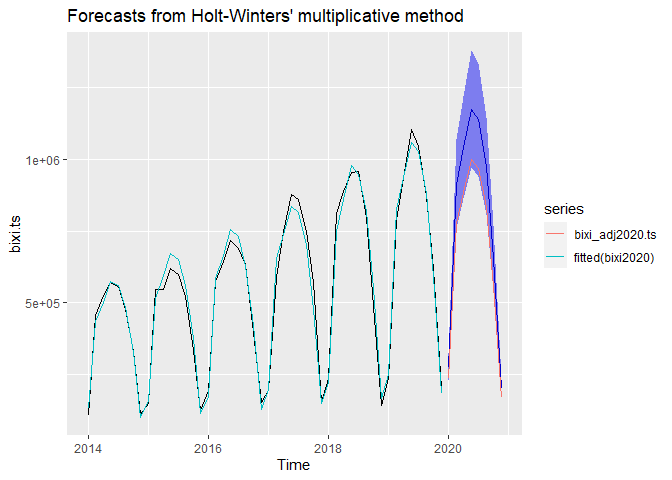
As we can see the adjusted forecast is too close to the lower boundary of the confidence interval of the forecast. However, we could have further worsened it by taking other factors into account: students that stopped commuting to school, employed people that no longer commute to work as they are working from home, for example.
Recommendations
1) BIXI should look towards the lower boundary of the forecast’s confidence interval because not so many people are going to ride BIXI’s.
2) Even though it may happen that the rides will drop considerably, BIXI should not close many of its stations because then people’s preferred routes will be disrupted. The only decisions they can make in the COVID-19 conditions should be regarding their workforce, maintenance and station “refill” schedules.
3) The forecast should be rerun as soon as new data becomes available to adjust for the constantly changing conditions.
Update
BIXI made their 2020 data available and it showed that even the downward adjusted forecast was too optimistic! Pretty much, after the adjustment, I should have just halved the number of rides given in the forecast.
#Importing the 2020 file
bixi2020 <- read.csv("OD_2020.csv")
bi20 <- bixi2020[!bixi2020$duration_sec<300,]

#Creating a new date
class(bi20$start_date)
bi20$start_date <- as.Date(bi20$start_date)
bi20$Month <- make_date(year(bi20$start_date), month(bi20$start_date),1)

#Counting rides per month
bi20 %>% group_by(Month) %>% count()
These are the actual values that I placed near the forecasted ones:
##    Period   Forecast    Adj_FC  Actual
## 2020-04-01  276057.2  235115.8  60574
## 2020-05-01  913586.4  778094.7  332185
## 2020-06-01 1040052.3  885804.7  478694
## 2020-07-01 1175116.0 1000837.4  557252
## 2020-08-01 1137016.2  968388.1  521514
## 2020-09-01  975976.7  831232.0  447204
## 2020-10-01  655910.0  558633.6  280374
## 2020-11-01  202177.9  172193.4  118959
Such a huge difference between the number of actual and forecasted rides is interesting. First of all, it shows by how much the habits changed in the COVID-19 year. Riding BIXIs was pretty common in the previous years, but in 2020, definitely, it was not so. Mainly, of course, because there were not so many places where people could ride. In addition, there could have been a way fewer tourists than estimated. Most of the rides were done by non-members the majority of who may be tourists. Thus, we can asssume that the drop in tourism was huge, which, definitely, hurt BIXI’s bottom line even though they claim that 2020 was a profitable year for them.
The actual data show the same pattern - the number of BIXI rides dropped almost twice to the previous year - as we can see in the graph! It is not really surprising why even the adjusted forecasts were overly optimistic!
Hopefully, BIXI will start a gradual recovery from the plunge in 2021!