Importing and Cleaning Kickstarter Data with R

Why Kickstarter?

If you need to find funds to realize your idea, Kickstarter may be an option for you being an all-or-nothing crowdfunding platform. There is a catch, though! Only those projects that have reached their monetary goal threshold will get the pledged money.

I find the Kickstarter platform to be a place where a lot of drama unfolds in front of our eyes. Each project is not just another observation in a dataset, but it is hours of hard work and thought and each project’s success or failure is someone’s tears of happiness or shattered dreams. The Kickstarter data tell a story of failures and successes, ups and downs and I want to know more about that story.

Task

This post’s main task is to describe the data preparation process. My further posts will be looking at the Kickstarter data from different angles and will be attempting to get answers to various questions, i.e. “Is Kickstarter a Worthy Option for a Project Funding?” and “What Projects Succeed on Kickstarter?”. It is going to be a long data analysis, data visualization and data modelling journey, but the answers and insights we will be getting during it are going to be worth it! Let the journey begin!

Where does the Data Come from?

I got the data from Webrobots. They started scraping data in April 2014, but it was done once every few months. Beginning in March 2016 Webrobots.io started collecting data on a monthly basis.

How many Sets were Available?

There were 69 zipped folders in total. 2014: 4 sets (April, August, October, December; JSON format) 2015: 6 sets (April, June, August, October-December; JSON and csv formats) 2016: 11 sets (March-December; csv format) 2017-2020: 12 sets each (January-December; csv format)

What Variables Did I Have?

Data were collected in multiple ways and the number of variables collected differed! So, the main focus for me was to find which variables were collected constantly throughout these 7 years to make sure that I could later create a master file for the above indicated timespan. Here are the variables that were the same for all years:

• id (project Id)
• creator_id (creator Id)
• name (project name)
• blurb (project description)
• backers_count (number of people who supported the project)
• goal (goal amount in the local currency)
• pledged (amount actually collected)
• currency (local currency)
• country (country where the project was created)
• city (city where the project was created)
• state (state where the project was created)
• created_at (when the project was created)
• launched_at (when the project was launched)
• deadline (when the money collection had to stop)
• state_changed_at (when the project was cancelled, named successful or something else)
• category (category the project was launched in)
• subcategory (subcategory the project was launched in)
• project_state (if the project was live, cancelled etc.)

What Variables did I Add?

Later I created additional variables:

• status (successful or failed)
• projectDays (number of the project duration in days: deadline - launched_at)
• dateScraped (an artificial date to help with removing duplicated projects later)
• mean_USD_rate (some local currency vs USD, calculated on a monthly basis, starting from January 2009)
• goal_USD (goal in the local currency * mean_USD_rate for that month and year)
• pledged_USD (amount pledged in the local currency * mean_USD_rate for that month and year)
• pledgedOverGoal (index of pledged_USD/ goal_USD)
• pledgedPerBacker (pledged_USD/backers_count)

How was the Data Imported?

I applied the following procedure: Unzip all files -> Import the data into R -> Bind all files for one month together (needed for csv files) -> Create a csv file for the appropriate month and year on the computer hard drive -> Once all the months have been recorded on the hard drive, bind them together to create a master file for all years -> Delete all duplicate rows -> Create a master csv file for further reference and analysis.

Webrobots store their data in a zipped format on their site. Each JSON object folder contains only one file, but each zipped folder with csv files has multiple csv files (30+) that need to be appended to represent a month of data. This makes manual data importing an impossible task also prone to multiple errors. Given different formats of the data, data reading had to be approached differently for JSON and csv files.

• CSV files: I created a folder called kickstarter. In that folder I created folders for each year of the csv data, i.e. 2015, 2016 etc. In each year I downloaded monthly zipped csv files. I did not unzip them.
• JSON files: In the kickstarter folder I created a folder called json_files14_15. In it I also added folders for each year of the JSON data (2014 and 2015) where I later placed zipped JSON files in their respective years. I did not unzip them either.

How were JSON Files Imported?

The 2015 October archive file had the .gz extension. I had to save it to zip so that all files had the same extension. Then everything was ready for the data import. At first I created a loop to unzip all the JSON data archives:

#Importing the library
library(plyr)
#WORKING WITH JSON DATA
#UNZIPPING JSON FILES
for(x in 2014:2015){
  mydir <- paste("D:/kickstarter/json_files14_15", x,sep="/")
  zip_file <- list.files(path=mydir, pattern="*.zip", 
                                    full.names=T)
  
  for(i in 1:length(zip_file)){
    dir.create(file.path(mydir, i))
    setwd(file.path(mydir, i))
    ldply(.data=zip_file[i], .fun=unzip, 
          exdir=paste(mydir,i,sep="/"))
  }
}

In total 8 JSON sets were imported:

• 2014: April, August, October, December
• 2015: April, June, August, October

It was really easy to import all 2014 and April 2015 JSON files because all the files’ structure was the same and there was nothing in the data that had to be fixed. For 2014 I created a loop to read all 2014 files and create monthly csv files on the hard drive. The full code is available in my GitHub repository.

#Importing the libraries
library(jsonlite) #to read JSON
library(tidyr) #to unnest JSON and turn into a rectangular format
library(stringr) #to work with strings 
year <- 2014
mydir <- paste("D:/kickstarter/json_files14_15",year,sep="/")
zip_file <- list.files(path=mydir, pattern="*.zip", 
                                        full.names=T)
for(x in 1:length(zip_file)){
mydir <- paste("D:/kickstarter/json_files14_15",year, x,sep="/")
setwd(mydir)
  
#creating a variable that retrieves a month value from a file name
date_month <- substr(sub(".*/","",zip_file[x]), 18,19)

#getting the file name
file <- sub(".*/","",list.files(path = mydir, pattern="*.json", 
                                        full.names=T))
  
#reading the JSON file
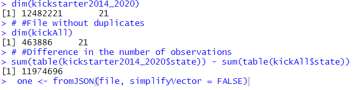
one <- fromJSON('Kickstarter_Kickstarter.json', 
                  simplifyVector = FALSE)
  
#unnesting lists (tidyr library)
kick <- tibble(data=one) %>% unnest_wider(data) %>% 
        unnest_longer(projects) %>% unnest_wider(projects)
  
#extracting and renaming creator id
creator <- tibble(creator = kick$creator) %>% 
                                      unnest_wider(creator)
creatorId = as.data.frame(creator$id)
kick$creatorId <-  creatorId$`creator$id`
  
#renaming variable state to condition (because I would like 
#the variable state to represent a location)
names(kick)[names(kick) == "state"] <- "condition"
  
#extracting location data
localization <- tibble(localization = kick$location) %>% 
                              unnest_wider(localization)
city = as.data.frame(localization$name)
kick$city <- city$`localization$name`
region <- as.data.frame(localization$state)
kick$region = region$`localization$state`
  
#extracting categories and subcategories
cat <- tibble(category=kick$category) %>%  
                              unnest_wider(category)
subcat <- as.data.frame(cat$name)
kick$subcategoryName <- subcat$`cat$name`
  
kick$categories <- str_extract(cat$slug, "[[:alnum:]\\s&]+")
}
}

The April 2015 file had no issues, but the 2015 June and August files were different. I kept getting errors when I tried to read them because the JSON data itself was corrupt. So, I had to open the JSON files using Windows Notepad and fix the following issues:

• Commas were missing in the array so I had to add them.

  # Error: parse error: after array element, I expect ',' or ']'
  # 7&ref=category&seed=2390189"}{ "projects": [  {   "id": 1699
  #                      (right here) ------^
  

• These brackets [ ] were found in the blurbs and names of some projects, and they triggered an error forcing fromJSON() to think that it was the end of the file. I had to remove them.

  # Error: parse error: premature EOF
  # [
  #   (right here) ------^
  

• At the end of the file an empty line was missing. So I had to go all the way to the end of the file and press Enter.

After those issues had been solved, the data was read in the same way as the 2014 (see the full code in my GitHub repository).

The October 2015 file, however, was a different fruit :) It represented just rows of data in the JSON format. So, the file had to be read in a different way. I applied a different code to import it:

year <- 2015
mydir <- paste("D:/kickstarter/json_files14_15",year,sep="/")
zip_file <- list.files(path=mydir, pattern="*.zip", full.names=T)
x<-4
mydir <- paste("D:/kickstarter/json_files14_15",year, x,sep="/")
setwd(mydir)
  
#creating a variable that retrieves a month value from a file name
date_month <- substr(sub(".*/","",zip_file[x]), 18,19)
  
file <- sub(".*/","",list.files(path = mydir, pattern="*.json", 
                                                    full.names=T))

#reading JSON lines
out <- lapply(readLines(file), fromJSON)

#unnesting JSON
one <- tibble(data=out) %>% unnest_wider(data) %>% 
                    unnest_wider(data)%>% unnest_longer(projects) 

#the projects' column contains dataframes, not lists
kick <- one$projects 

#extracting and renaming creator id from the dataframe
kick$creatorId <- kick$creator$id

#renaming variable state to condition (because 
#I would like the variable state to represent a location)
names(kick)[names(kick) == "state"] <- "condition"
  
#extracting location data
kick$city <- kick$location$name
kick$region <- kick$location$state

#extracting categories and subcategories
kick$subcategoryName <- kick$category$name
kick$categories <- str_extract(kick$category$slug, 
                                      "[[:alnum:]\\s&]+")

Only a part of the code is presented here. The full code used can be found in my GitHub repository.

How were CSV Files Imported?

Even though JSON files were available for all months, I opted for csv because they were much faster to import and save. Say, the July 2019 folder contained 57 files. It took R studio only 3 minutes to import those files into R, append them to each other and save them as a single July2019 csv file on my computer. Reading JSON files took a way longer. To read all 61 zipped archives with csv files and then save them as csv monthly files I created two loops:

• One loop - to unzip the files:

for(x in 2015:2020){
  mydir <- paste("D:/kickstarter",x,sep="/")
  zip_file <- list.files(path=mydir, pattern="*.zip", 
                                        full.names=T)
  for(i in 1:length(zip_file)){
    dir.create(file.path(mydir, i))
    setwd(file.path(mydir, i))
    ldply(.data=zip_file[i], .fun=unzip, 
          exdir=paste(mydir,i,sep="/"))
  }
}

• The other loop - to read, append and save files:

#READING, CLEANING AND MERGING SETS FOR YEARS: 2015-2020
#USING A FOR LOOP
for(year in 2015:2020){
  mydir <- paste("D:/kickstarter",year,sep="/")
  zip_file <- list.files(path=mydir, pattern="*.zip", 
                                    full.names=T)
for(x in 1:length(zip_file)){
mydir <- paste("D:/kickstarter",year, x,sep="/")
setwd(mydir)

#creating a variable that retrieves 
#a month value from a file name
date_month <- substr(sub(".*/","",zip_file[x]), 18,19)

#reading csv files in batch
kick <- do.call(rbind, lapply(list.files(path = mydir, 
             pattern="*.csv", full.names=T), read.csv))

#The code used to create or clean columns, bind columns 
#and so on is missing in this code snippet
}
}

Only a part of the code is represented here. The full code can be accessed in my GitHub repository.

What Issues did I Have to Solve with the Loops?

The JSON data could be easily imported “manually” as it only contained 8 files, but the csv zipped folders represented the biggest challenge

• There were 61 zipped files available

• Each zipped folder contained 40+ files, which had to be appended

Unzipping and importing them manually meant making multiple errors on the way without even realizing it! That is why using loops was inevitable.

• Unzipping csv files was the same as for the JSON data (library(plyr)):

I created two loops: the outer FOR-loop initiates an iteration for a specific year, the inner FOR-loop creates a folder for a specific month while the ldply function unzips files into that folder. After the inner loop is done with all the months in that year, it goes to the next year. FOR-loops I created had to be flexible because the year of 2015 had 2 month, the year of 2016 - 11, while 2017-2020 had 12 months which made it impossible to define a fixed range for the inner loop.

To resolve the issue, I created a list of all zip files per year, the number of elements in which corresponded to the number of months in a specific year. Instead of specifying the maximum of the range, I used the length() function. It just returns a value that represents a number of elements in a list. It allowed me make the loop flexible since the maximum value of range always depended on the number of zip files in the list. The code with comments is presented below.

#Importing the library
library(plyr)

#Creating the loops
#The outer loop for years that also creates 
#a directory and a list of .zip files in it
for(x in 2015:2020){
mydir <- paste("D:/kickstarter",x,sep="/")
zip_file <- list.files(path=mydir, pattern="*.zip", 
                                      full.names=T)
#The inner loop specifies the maximum range value
#to equal to the number of elements
#in the list of zip files for a specific year
  for(i in 1:length(zip_file)){
    dir.create(file.path(mydir, i)) #Create a directory
    setwd(file.path(mydir, i)) #Assign a directory
    ldply(.data=zip_file[i], .fun=unzip, 
          exdir=paste(mydir,i,sep="/")) 
#Batch process files with .zip extension
  }
}

• Assigning Unique Names to Newly Created Files in the Loops

  I saved each merged month of data as a csv file in the kickstarter folder. Since all monthly csv files had to be located in the same folder, I had to make sure that each newly created file had a unique name. In the outer loop I created a vector called zip_file that contained a list of names of all zipped files for a specific year. Within the name of each zip file a year-month-day value was included. All I had to do was to extract the value of the month and use it when I named my merged csv file. So, the steps were like that:

1) Create a list of zip files for a specific year in the outer loop:

#The outer loop for years that also creates a directory 
#and a list of .zip files in it
for(x in 2015:2020){
  mydir <- paste("D:/kickstarter",x,sep="/")
  zip_file <- list.files(path=mydir, pattern="*.zip", 
                  full.names=T) 
#a list of zip files for a specific year
  }

2) In the inner loop extract a month value:

• When the inner loop starts, it will look at the corresponding index in the zip_file vector and will retrieve the name of the zip file from the list available there under that index. The substr() function from the stringr library will retrieve the values at a specific position in the string. For example, the second iteration in the year of 2016 will lead us to a zipped file with this name: Kickstarter_2016-03-22T07_41_08_591Z The value of the month can be retrieved from the location 18-19.

library(stringr)
date_month <- substr(sub(".*/","",zip_file[x]), 18,19)
#Here I am deleting everything before the final 
#slash and retriving the value of the month 
#at the position 18,19

• Paste that value together with the year to generate a date composed of year, month, day (01).

#generating the date
generated_date <- paste(year, date_month, 01, sep="-")

• Retrive a name of the month associated with it by applying a specific format:

#extracting the word month name from the date
dates <- format(as.Date(generated_date), "%B")

• Combine the word name of the month, the year and the csv extension to create a file name.

a <- paste(dates, year, ".csv", sep="")

• Record a csv file from the merged csv for March 2016. The code below is given just for demonstration purposes. I extracted it from a much bigger chunk of code given at the end of the post.

write.csv(kickstart, paste("D:/kickstarter", a,sep="/"), 
                                      row.names = FALSE)

The full code can be accessed in my GitHub repository.

• Adding Variables to the Set

  Between the data import and saving the monthly files as csv, I created additional variables - status (of the project) and projectDays:

#if the project was successful or not. 
#Successful projects are the ones that reached or exceeded goals
status = as.character(ifelse (kick$pledged>=kick$goal, 
                                       "successful", "failed"))

#how many days the project lasted from 
#the launch date to the deadline
kickstart$projectDays <- difftime(kickstart$deadline,
                           kickstart$launched_at, units="days")

How Were the Data Cleaned and Transformed?

• Timestamp in the UNIX Format

  The UNIX date is not readable by humans and looks like that: 1368652795. According to Wikipedia, Unix time is “the number of seconds that have elapsed since the Unix epoch, minus leap seconds; the Unix epoch is 00:00:00 UTC on 1 January 1970”. Here are the steps I had to take to make them readable by us:

• Make sure the UNIX timestamps are numeric

• Apply the as.POSIXct() function to transform the output to the standard human datestamp output

• Use the as.Date() function to return the result as a date.

The code below is given just for demonstration purposes. The full code can be accessed in my GitHub repository.

kickstart$created_at <- as.Date(as.POSIXct(as.numeric(as.character(kick$created_at)),
                                                              origin="1970-01-01"))

• Some Columns Contained Values to be Assigned to Various Variables

  Some cells contained loads of data, some of which can be useful and can provide some insights into projects’ success on Kickstarter. Four columns contained redundant text with values that had to be assigned to multiple variables. These columns were:

• category, from which category and subcategory name could be extracted

• location, from city and region/state could be extracted

• creator, from which creator id could be retrieved

• profile, from which project state (active/inactive) could be gotten

I discarded the idea of splitting the columns by a specific separator because the process took a long time and was inefficient. I decided to retrieve data from the strings into specific variables right away. At the beginning, to each string I applied the sub() function to delete all the text before and including a specific word to make sure that the data I wanted to extract would be in the first position. Then I applied the str_extract() function from the stringr package to extract a specific value.

For instance, for the category names I deleted all the preceding text including “slug” and gave str_extract() an instruction to retrieve all alphanumeric values with spaces and &: “[[:alnum:]\s&]+”. The ‘+’ sign allowed for flexibility as the number of characters to extract varied. To get the creator id, I deleted everything preceding and including the word “id” and then retreived only digits by using str_extract() and the regular expression “\d+” as an argument. Here is an extract of the code for the new variables that I created based on the two columns described above.

#retrieving needed values, cleaning the data
kick$categories <- str_extract(sub(".*\"slug\"","",kick$category), 
                                              "[[:alnum:]\\s&]+")

kick$creatorId <- str_extract(sub(".*\"id\"","", kick$creator), 
                                                          "\\d+")

It took only 2-3 minutes until the newly created csv file was saved! Only slightly above 2 hours were needed to process and save all the files! It’s almost 14 times less hours than was required to save csv’s when columns were split!

• Duplicated Projects

  Some projects lasted for months and thus, they would be found in different monthly sets. To avoid double, triple or n-times counting, duplicates had to be removed. Taking into account that we only had deadline, launched_at, created_at and state_changed_at dates available, it wasn’t really helpful. Since one project could last for months, the crawler would keep scraping it on a monthly basis, adding multiple records of the same project to the master set. So, to resolve the issue, I decided to use the following approach:

1) Generate a date that would correspond to the month and year when the set was scraped like in the example below. The date_month variable was described above. Its value comes from the date portion of the zip archive’s name.

#The year is generated in the outer loop and the date_month 
#is retreived from the month's value from 
#the zip file name as described above
kickstart$dateScraped <- as.Date(paste(year, date_month, 01, 
                                                    sep="-"))

2) Merge all sets into a master set.

#Setting the new directory
mydir <- "D:/kickstarter"

#Merging all the files
kickstarter2014_2020 <- do.call(rbind, 
        lapply(list.files(path = mydir, pattern="*.csv",
                               full.names=T), read.csv))

3) Sort the id column in any order and sort the dateScraped in the descending order.

#Changing the date variable to class date
kickstarter2014_2020$dateScraped <- as.Date(kickstarter2014_2020$dateScraped)

#Sorting the set by projectId and date
newSet  <- kickstarter2014_2020[order(kickstarter2014_2020$id, 
        kickstarter2014_2020$dateScraped, decreasing = TRUE),]

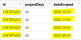
4) Keep only the most recent id.

#Keeping rows that are not duplicated
kickAll<- newSet[!duplicated(newSet$id), ]

As can be seen in the image, removing duplicate ids has decreased the number of observations considerably! By almost 12 million rows!

5) If necessary, the file may be saved as a csv file. It is not the final version of the file yet.

#Saving the full file for further work
write.csv(kickAll, "D:/kickstarter/kickAll.csv", 
                                    row.names = FALSE)

• Adding Currency Exchange Rates and Other Variables to the Set

  The goal and pledged amounts were given in the local currency, which made comparison of projects from different countries impossible. I checked what currencies were present in the Kickstarter data and found those currencies vs USD average monthly exchange rates beginning from the 2009 at ofx.com. Here is the procedure I followed:

• Create a table with dates and average currency rates vs USD (a csv file)

• Import that table into R

#ADDING CURRENCY EXCHANGE VALUES TO THE KICKSTARTER DATA
#IMPORTING A CSV FILE
currency <- read.csv("D:\\kickstarter\\extra_files\\currency.csv", 
                                            stringsAsFactors = F)

#Renaming the date variable
names(currency)[1] <- "date"

• Pivot it using the tidyr package to get currency column names in the column named “currency” and the currency exchange rates in the column called “rate”

#Pivoting the currency table to get 
#the column names into the column levels
currency_pivot <- currency %>% pivot_longer(-date, 
            names_to="currency", values_to="rate", 
                              values_drop_na=TRUE)

• Create a date column so that each month begins on the first day, i.e. 2009-01-12, etc.

#Changing the date format
currency_pivot$date <- dmy(currency_pivot$date)

#Creating a date with the first day of each month
year <- year(currency_pivot$date)
date_month <- month(currency_pivot$date)
generated_date <- paste(year, date_month, 01, sep="-")
currency_pivot$currency_date <- as.Date(generated_date)

#drop the first column
currency_pivot <- currency_pivot[,-1]

• In the master set create a date column based on the projects’ launched_at dates, but each date should also start on the first day of the month.

#create a date that starts with the first day of the month
#will be used as a part of the composite key
#together with the currency exchnage
kickstarter_data$launched_at <- as.Date(kickstarter_data$launched_at)

#Generate the date based on the launched at date
year <- year(kickstarter_data$launched_at)
date_month <- month(kickstarter_data$launched_at)
generated_date <- paste(year, date_month, 01, sep="-")
kickstarter_data$currency_date <- as.Date(generated_date)

• Use the currency (with local currency names) and the newly created columns with dates as a composite key for the left join (the kickstarter master set is the left set).

#Merging two sets
kickstarter_all <- kickstarter_data %>% left_join(currency_pivot, 
                              by = c("currency_date", "currency"))

• Add new variables I created goalUSD and pledgedUSD for easier comparison across projects. I also created PledgedOverGoal variable to see by how much the pledged amount was different from the goal amount and pledgedPerBacker to see what average sum was pledged by a backer.

kickstarter_all$goalUSD <- round(kickstarter_all$goal*kickstarter_all$rate,2)
kickstarter_all$pledgedUSD <- round(kickstarter_all$pledged*kickstarter_all$rate,2)
kickstarter_all$pledgedOverGoal <- round(kickstarter_all$pledgedUSD/kickstarter_all$goalUSD,4)
kickstarter_all$pledgedPerBacker <- round(kickstarter_all$pledgedUSD/kickstarter_all$backers_count)

• Save the new data

#SAVING THE FINAL SET - WITH THE USD DATA
write.csv(kickstarter_all, "D:/kickstarter/kickFull.csv", 
                                        row.names = FALSE)

How was the Final Set Created for Further Analysis?

For the analysis, I did not want to include any projects whose deadline had not been reached before the data were scraped in December 2020. So, the projects whose deadline was on the 17th of December 2020 or later were discarded. The projects that were cancelled or suspended were also discarded. The resulting set was recorded and saved for further analysis!

#CREATE A SET FOR ANALYSIS
#SUBSETTING THE FOLLOWING WAY:
#- CUT OFF DATE - BEFORE THE FINAL SET WAS SCRAPED
#- NOT CANCELED AND NOT SUSPENDED
#Subsetting the data to only contain
kickSuccess <- subset(kickFull, 
      deadline < as.Date(paste(2020, 12, 17, sep="-")) &
      project_state != "canceled" & project_state != "suspended")

#Checking if subsetting worked
table(kickSuccess$project_state)

#Saving the file for further reference - all the work
#will be done with this file
write.csv(kickSuccess, "D:/kickstarter/kickSuccess.csv", 
                                        row.names = FALSE)

Finally, after the boring part was over, the data were ready for the analysis! You can access the full code in my GitHub repository.